Solving differential equations numerically. Part 1: SciPy’s solve_ivp

The hallmark of a differential equation is that it describes the rate of change, typically over time. Here is a most simple case of a decay process (as in radioactive decay) where we start with a quantity $N_0$ which decays in proportion to the amount of N at any given time with $k$ being the (negative) proportionality factor:

   

This indeed very simple specimen is a first order ordinary differential equation (ODE). ‘First order’ because we don’t have any higher derivatives like

   

and ‘ordinary’ just because it is not a partial differential equation.

We could certainly solve this ODE analytically. The separation of variables is a method to do that and is described in detail here. But right now we are only interested in solving the ODE numerically. Could by done by hand (e. g. with Euler’s method), but this is tedious work, which is best relegated to a computer. Scripting the necessary computer program from scratch (e. g. by implementing Euler’s method) could be a worthwhile undertaking, but others have already come up with ready-made algorithms that, in addition, cover a wide range of applications even when a basic approach would quickly run aground. In the Python ecosphere, such an algorithm is the function solve_ivp from the Scipy library. ‘ivp’ stands for initial value problem. As mentioned above, we start with known quantity in the beginning, and this is the initial value.

How does solve_ivp look like and how is it to be used? Here is what the official documentation has to say:

scipy.integrate.solve_ivp(fun, t_span, y0, method='RK45', t_eval=None, dense_output=False, events=None, vectorized=False, args=None, **options)

Looks impressive and somewhat forbidding. And the rest of the documentation is unfortunately not always entirely helpful. But it is not that difficult to get started. Instead of describing all the constituent parts of this function in minute detail, it is best to dive right in. The additional bits and pieces can be filled in on the way.

First, we need to import the necessary libraries. Numpy (as practically always), and to put out the results graphically Matplotlib. And from the Scipy library we fetch specifically solve_ivp:

import numpy as np
import matplotlib.pyplot as plt
from scipy.integrate import solve_ivp

Now we set up the differential equation from above

   

and we start with an initial value of, say, $N=1000$ (e. g. decaying atoms), which we want to observe over a time interval of 100 time units. The proportionality factor shall be $k=-0.1$.

Let’s start with the easiest step, defining the proportionality factor $k=-0.1$. It is a simple number.

k = -0.1

The next step is setting up the differential equation in a form that can be fed into solve_ivp. This is done by defining a function (in the usual Python way):

def function1(t, N):
    return k*N

• function1 is just an arbitrary name. Could be anything.
• Function arguments (t, N): N is our system variable from the ODE above. t stands for time. Note two things here: 1) Time must be the first argument in the parentheses. 2) t and N are only variable names. You can choose any other names (as long as you are consistent).
• return k*N: In this line the differential equation is finally defined. But where is the $dN/dt$ part? Well, it is simply not needed. The right hand side of the equation says it all. (Sometimes you may find the entire function written out complete with an equal sign between the left and the right side, and this is just as fine.)

With that everything we need is already set up. Time for the solver:

sol = solve_ivp(function1, [0, 100], [1000])

Again, this looks more complicated than it actually is:

• sol is an arbitrary variable name for the solution.
• At its core solve_ivp needs three arguments. 1) Which differential function to solve (defined as function1 above). 2) [0, 100] states the time interval. Here it starts at 0 and ends at 100. 3) [1000] looks like the initial value of $N=1000$, and indeed it is.

Running this line puts the solution of our differential equation into the variable sol. To see how it looks like we print it as a graph:

plt.plot(sol.t, sol.y[0])
plt.xlabel('t')
plt.ylabel('N')
plt.show()

The solution variable sol has a specific inner structure. The time vector is always accessed through the attribute t, and the solution vector comes always as y, no matter how we name the system variable. The first system variable (and in our case here, the only one) is stored under the first index ([0]) of sol.y (which is not a vector but an array).

That is it. The differential equation describing exponential decay solved numerically.

Here is the script in its entirety:

k = -0.1

def function1(t, N):
    return k*N

sol = solve_ivp(function1, [0, 100], [1000])

plt.plot(sol.t, sol.y[0])
plt.xlabel('t')
plt.ylabel('N')
plt.show()

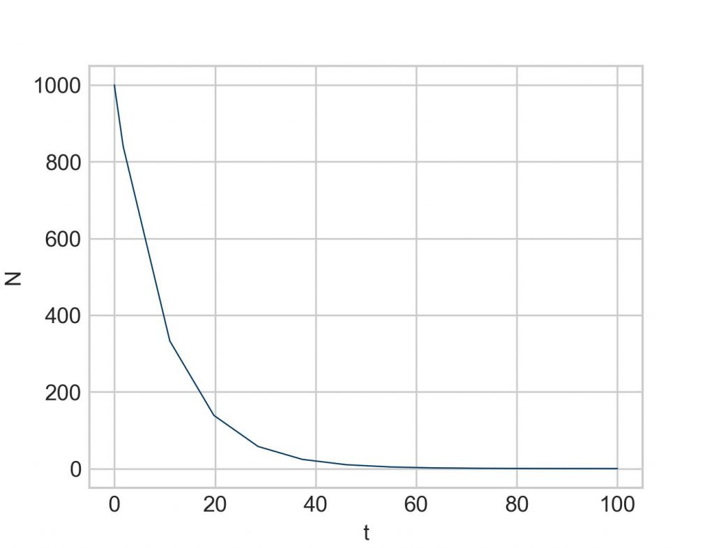
But wait, you say. The plot looks oddly jerky. Shouldn’t it be a smooth exponential curve?

Correct. The only problem is that without giving additional instructions to solve_ivp, it decides for itself how many points to calculate, and the default mode is apparently not up to our (due) expectations.

Let’s check how many data points we have by looking at the time vector sol.t:

print(sol.t)
print('Vector length: ', len(sol.t))

[  0.           0.15848935   1.74338286  11.01708551  19.77576922
  28.56631307  37.35488334  46.14359414  54.93233916  63.72118548
  72.51027441  81.29994729  90.09102515  98.88548141 100.        ]
Vector length:  15

Note that the time vector starts at 0 and ends with 100, just as we defined.

To coax solve_ivp into producing more data points we have several options. The by far most common one is stating the time points explicitly at which we want to get a result. For this solve_ivp accepts an additional argument, called t_eval. Into this argument we can put any sequence of numbers as long as its start and end conform with the values of the already defined time interval (and it must be a strictly ascending sequence). I typically use the Numpy function np.linspace(), which spaces out the desired number of numbers evenly over the interval. solve_ivp went for 15 time points. Let’s increase the value to 100 and see how the resulting plot looks:

sol = solve_ivp(function1, [0, 100], [1000], t_eval=np.linspace(0, 100, 100))

plt.plot(sol.t, sol.y[0])
plt.xlabel('t')
plt.ylabel('N')
plt.show()

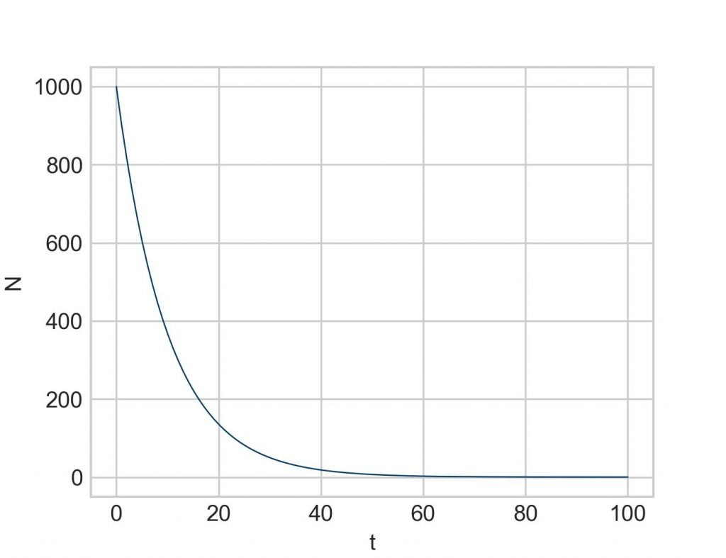
Much better.

Checking the length of the time vector:

print('Vector length: ', len(sol.t))

Vector length:  100

Please note that with that we use the values for the interval start and end more than once in the script. If you wished to modify the parameters, you would have to do this everywhere the parameters occur. This is an invitation for errors. Therefore, it is best to define values only once, and use them as variables later. And while we are at it, it is advisable to tuck all the parameters together in one corner, including the initial value of 1000 (here with the highly sophisticated variable name iv):

k = -0.1
iv = 1000
start = 0
end = 100

def function1(t, N):
    return k*N

sol = solve_ivp(function1, [start, end], [iv], t_eval=np.linspace(start, end, 100))

Or even more condensed by using a list:

k = -0.1
iv = 1000
interval = [0, 100]

def function1(t, N):
    return k*N

sol = solve_ivp(function1, [interval[0], interval[1]], [iv], t_eval=np.linspace(interval[0], interval[1], 100))

And for the ultimate pros, a list can be conveniently accessed item by item using the star or asterisk sign $*$:

k = -0.1
iv = 1000
interval = [0, 100]

def function1(t, N):
    return k*N

sol = solve_ivp(function1, [*interval], [iv], t_eval=np.linspace(*interval, 100))

But for now we will stick to start and end because it is a tad more readable.

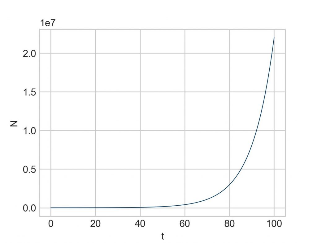
In any case, this is how to use Scipy’s solve_ivp to solve a differential equation (or a system of multiple differential equations, which we will cover later in another post). With this basic structure we can investigate all the differential equations that might be of interest. Why not try out exponential growth instead of exponential decay above? Simply change the sign of k to positive:

k = 0.1
iv = 1000
start = 0
end = 100

def function1(t, N):
    return k*N

sol = solve_ivp(function1, [start, end], [iv], t_eval=np.linspace(start, end, 100))

plt.plot(sol.t, sol.y[0])
plt.xlabel('t')
plt.ylabel('N')
plt.show()

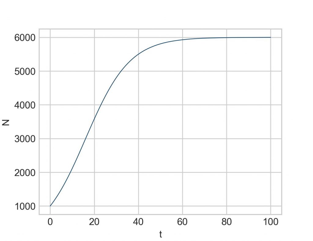
Or perhaps logistic growth as described by the following differential equation:

   

with the new parameter C to denote the carrying capacity of the system:

k = 0.1
iv = 1000
C = 6000
start = 0
end = 100

def function1(t, N):
    return k*N*(1 - N/C)

sol = solve_ivp(function1, [start, end], [iv], t_eval=np.linspace(start, end, 100))

plt.plot(sol.t, sol.y[0])
plt.xlabel('t')
plt.ylabel('N')
plt.show()

Further reading

• Barnes B, Fulford GR. Mathematical modelling with case studies. CRC Press 2015
• Gamsjäger T. Separation of variables. Maytensor 2025
• Logan JD. A first course in differential equations. Springer 2015
• Scipy Documentation. https://docs.scipy.org/doc/scipy/reference/generated/scipy.integrate.solve_ivp.html

Back matter

Copyright Thomas Gamsjäger

Cite as: Gamsjäger T. Solving differential equations numerically. Part 1: SciPy’s solve_ivp. Maytensor 2026

Featured image: This is the nuclear power plant in Zwentendorf, Austria. It is famous for the fact that after completion of construction in 1978 it was never activated.