Solving differential equations numerically. Part 2: Euler’s method

In the previous article, we used the ready-made algorithm solve_ivp from the Python library Scipy to numerically solve a differential equation. As happy we are that somebody else has shouldered the burden of programming such a neat solver so that we can put it to use to our heart’s content, wouldn’t be interesting to know how such a tool works, at least in principle?

If your answer is yes, it is good that you are here. You might be surprised how simple it is to solve a differential equation numerically with only a couple of lines of code.

Again, we start with a very simple ordinary differential equation, the one for describing exponential growth:

   

To solve this differential equation we need the value of the variable k and, of course, the first value N. It is an initial value problem (IVP) after all.

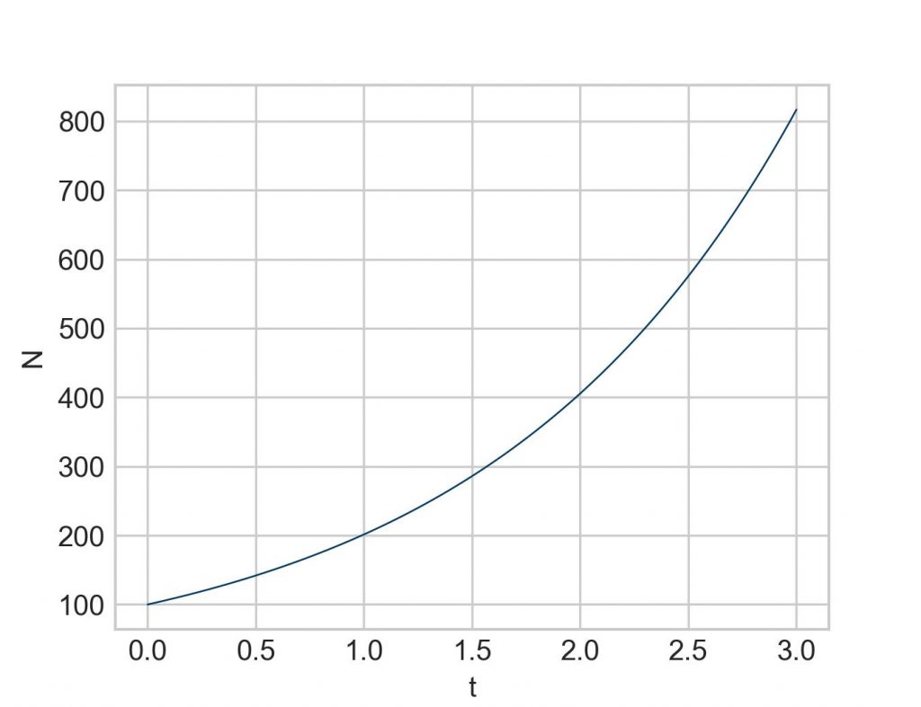
For everything that follows it is best to have a solid baseline. Why not use solve_ivp? Is at the same time a good opportunity to recap how it works:

import numpy as np
import matplotlib.pyplot as plt
from scipy.integrate import solve_ivp

k = 0.7
iv = 100
start = 0
end = 10

def function1(t, N):
    return k*N

sol = solve_ivp(function1, [start, end], [iv], t_eval=np.linspace(start, end, 100))

plt.plot(sol.t, sol.y[0])
plt.xlabel('t')
plt.ylabel('N')
plt.show()

Now to what Leonhard Euler, one of the greatest mathematicians of all time (1707-1783), has developed for us. Recall that the derivative of a function (at a certain point) is simply the rate of change of the function (at this point). And the rate of change is nothing but the slope of the graph (at this point). This is basically all we need to do some very basic calculations.

First, we calculate the rate of change (or slope) at time $t=0$ simply by plugging the values we know into the differential equation. Sounds counterintuitive, but trust me:

   

Note that this value is not an approximation. At time $t=0$ the rate of change is exactly $70$ (given the parameters we have). The tiniest amount of time later the value will be somewhat higher, but we don’t know by how much. Therefore, we pretend that the value remains constant for, say, one time unit. With that we can calculate the value at $time=1$ by taking the initial value of $N_0=100$ and adding the rate of change $dN/dt=70$ multiplied by the time interval $\Delta t=1$ (also often called stepsize). (In textbooks, $\Delta t$ is practically always denoted by $h$, but for now we will stick to $\Delta t$ as it is a bit clearer.)

   

This new value of 170 is our first approximation. Now we repeat the procedure with this new value while the other parameters ($k$ and $\Delta t$) remain unchanged:

   

   

Let’s do one more iteration:

   

   

Here is where these newly calculated points find themselves in the plot from above. Note that the straight lines between the points depict the slope that we have calculated at the beginning of each segment.

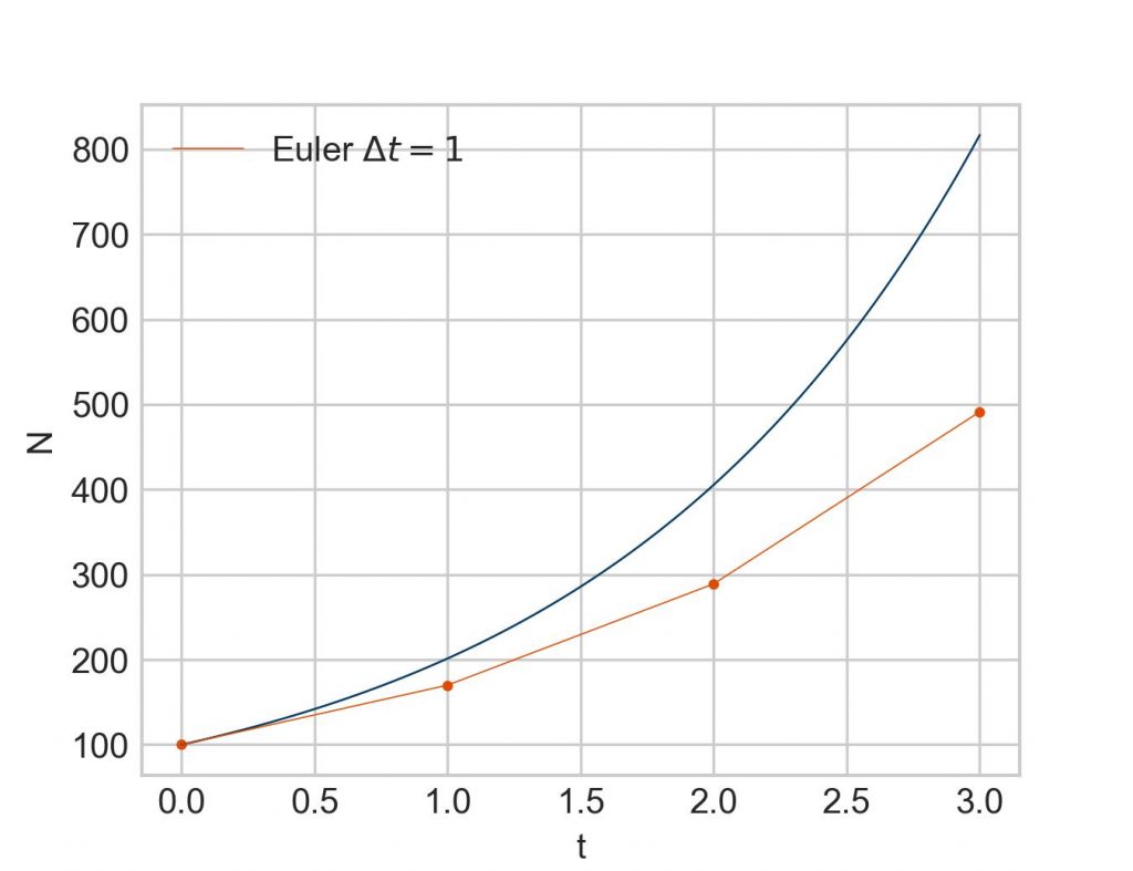
Admittedly, a crude approximation. Can we do better? Certainly. We have only to reduce the time interval $\Delta t$, e. g. to $\Delta t=0.5$:

   

   

Next iteration at $\Delta t=0.5$:

   

   

Next iteration at $\Delta t=1$:

   

   

If we keep going this way, we can set up the following table:

0	100	70	35
0.5	135	94.5	47.25
1.0	182.25	127.575	63.7875
1.5	246.0375	172.22625	86.113125
2.0	332.150625	232.5054375	116.25271875
2.5	448.40334375	313.88234062	156.94117031
3.0	605.34451406

But much more interesting is how the plot looks like:

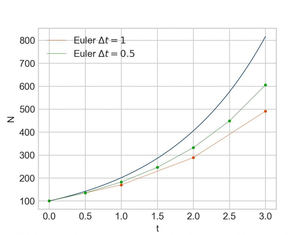
Apparently, a pattern begins to emerge. With more steps (= smaller stepsize), the approximation moves closer to true result. The flipside of that is that a whole lot more iterations have to be calculated. While everything can definitely be done with the help of a pocket calculator, already going from three calculated points to six (as given in the table above) makes abundantly clear that better tooling is needed, even more so with smaller and smaller stepsizes. Fortunately, for such task we have… computers.

Time for a Python script. As we are doing the same operation again and again, a for loop is the approach of choice. To simplify things we calculate $N$ without storing $dN/dt$ etc. $k$ shall be the same as above, but we go for 100 steps:

import numpy as np
import matplotlib.pyplot as plt

end = 3
steps = 100
k = 0.7

Nothing fancy so far.

delta_t = end/steps

N = np.zeros(steps+1)
N[0] = 100

time = np.arange(0, end+delta_t, delta_t)

These are additional preparatory elements. We calculate the stepsize by dividing the end time by the number of steps. Then we create a placeholder vector for N with np.zeros(steps+1)so that we can store the values the for loop will calculate for us in a minute. The +1 is necessary because we will calculate one N more than we have steps. And the time vector is needed to give us the correct time points for plotting the result. Now for the loop:

for i in range(steps):
    N[i+1] = N[i] + k*N[i]*delta_t

This is exactly what we have done above by hand. Ready to plot the result:

plt.plot(time, N)
plt.xlabel('t')
plt.ylabel('N')
plt.show()

In conclusion, even though Euler’s method is rarely implemented these days as more efficient variations have been developed (the Runge-Kutta method being one of the more prominent ones), Euler’s method is a powerful algorithm that is, at its core, simple enough to be executed by hand, a pocket calculator, and a bit of patience. But with the help of a short Python script practically any level of accuracy of the result can be achieved in solving any differential equation.

Further reading

• Barnes B, Fulford GR. Mathematical modelling with case studies. CRC Press 2015
• Feldman DP. Chaos and dynamical systems. Princeton University Press 2019
• Gamsjäger T. Solving differential equations numerically. Part 1: SciPy’s solve_ivp. Maytensor 2025
• Logan JD. A first course in differential equations. Springer 2015
• Sundnes J. Solving ordinary differential equations in Python. Springer 2024 (freely available from the publisher as an open access book here)

Back matter

Copyright Thomas Gamsjäger

Cite as: Gamsjäger T. Solving differential equations numerically. Part 2: Euler’s method. Maytensor 2026

Featured image: Portrait of Leonhard Euler by Jakob Emanuel Handmann, 1753. Public domain.